|
|
|
Materials and Methods
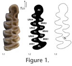
The right and left teeth of each individual were photographed with a Canon 350D digital SLR camera with macro lens arrangement giving x2 magnification. Care was taken to orient each tooth so that its occlusal surface was oriented horizontally, perpendicular to the line of sight. The left tooth of each individual was flipped to remove the effects of mirroring. The outline of each tooth was traced using image processing software (Adobe Photoshop CS2 ©). Chips in the enamel were ignored in the tracing because we did not want to include differences due to breakage in our estimate of asymmetry. Two hundred fifty evenly spaced points were then fitted to the traced outline for quantitative analysis. The points ran counterclockwise around each outline starting at the apex of the first buccal reentrant angle (Figure 1.3). We analyzed the coordinates using two different outline methods to ensure that choice of method did not substantially affect the results. The first method was Standard 2D Eigenshape (Lohmann 1983; MacLeod and Rose 1993; MacLeod 1999). In Eigenshape, the outline coordinates are transformed to a Zahn and Roskies (1972) shape function (φ), which is a vector of net angular change the positions of neighbouring outline coordinates beginning at an arbitrary starting position that is the same on all objects. The function was standardized by subtracting the angles describing a circle of the same mean radius (φ*) as recommended by MacLeod (1999). The tooth outlines were ordinated in principal components (PC) space by singular value decomposition of the covariance matrix of the φ* functions. The PC scores of the tooth outlines are, by definition, uncorrelated with one another but preserve the shape distances among the original outlines and so can be used as shape variables for further statistical analysis. Eigenshape distances between tooth outlines can be calculated either as the Euclidian distance between the φ* functions or as the Euclidean distance between the full set of PC scores (the two distances are identical). These distances are analogous to Procrustes distances in landmark analysis. The second method of shape analysis was a Procrustes-based semilandmark analysis (Bookstein 1991; Rohlf 1993; Dryden and Mardia 1998; Zelditch et al. 2004). The same 250 outline coordinates were treated as semilandmarks (Bookstein 1997). The shapes were superimposed using Generalized Procrustes Analysis (GPA, Rohlf 1990). The mean shape was subtracted from the superimposed coordinate points. The tooth shapes were ordinated in PC space by singular value decomposition of the covariance matrix of the resulting Procrustes residuals. Like with Eigenshape, the PC scores are uncorrelated and preserve the original shape distances and so can be used as shape variables for further statistical analysis. Procrustes distances between the tooth shapes can be calculated either as the Euclidean distances between their Procrustes superimposed coordinate points or as the Euclidean distance between the full set of PC scores for the two teeth. Shape variance was partitioned into between-individual and between-side components using Multivariate Analysis of Variance (MANOVA) on the PC score shape variables with both data sets for each of the four species. The between-individual component of variance is the part that describes the average difference between the teeth of individual voles independent of asymmetry; the between-side component describes the variance between left and right sides. The former is an estimate of within-species variance unbiased by the non-genetic variance associated with fluctuating asymmetry; the latter is a minimum estimate of environmental variance, E (Palmer and Strobeck 1985; Klingenberg and McIntyre 1998). The absolute values of the variance components are rather arbitrary since the scale differs between Eigenshape and Procrustes analysis. However, the proportions of between-individual and between-side variances to the total variance can be compared from one analysis to the other. A maximum estimate of heritability (h2), which is the proportion of phenotypic variance that is passed from parent to offspring, can be calculated as h2 = 1 – (between-sides variance / total variance), ( Equation 2) which is the same as h2 = G/P since the between-sides variance is a proxy for E. By Equation 1, G/P = 1 – (E/P). This estimate of h2 must be considered a maximum because some environmental variance will be undetected by the analyses presented here, as mentioned above. |
|